Multivariate Analysis of Transcript Splicing (MATS)
Xing Lab, University of California, Los Angeles
Install MATS:
|
|
|
|
|
|
|
|
|
cd
tar -xvzf MATS.2.1.0.tgzcd ~/bowtieIndexestar -xvzf bowtieIndexes.tgz
tar -xvzf MATS.2.1.0.tgzcd ~/bowtieIndexestar -xvzf bowtieIndexes.tgz
Test MATS:
Run testRun.sh as below to test MATS runs properly.
cd ~/MATS.2.1.0
./testRun.sh ~/bowtieIndexes/hg19
This two outputs can be found in the fastqTest and bamTest directories. The test run output should look like the MATS output description../testRun.sh ~/bowtieIndexes/hg19
Trim Fastq (Optional):
To trim the poor quality 3' end of reads, use the trimFastq.py script found in the bin directory.
python trimFastq.py input.fastq trimmed.fastq desired_length
cd ~/MATS.2.1.0/
python bin/trimFastq.py testData/231ESRP.250K.r1.fastq testData/trimmed.fastq 32
The above command trims 231ESRP.250K.r1.fastq to 32 bp long by removing sequence from the 3' end of the reads and then saves it to trimmed.fastq.
python bin/trimFastq.py testData/231ESRP.250K.r1.fastq testData/trimmed.fastq 32
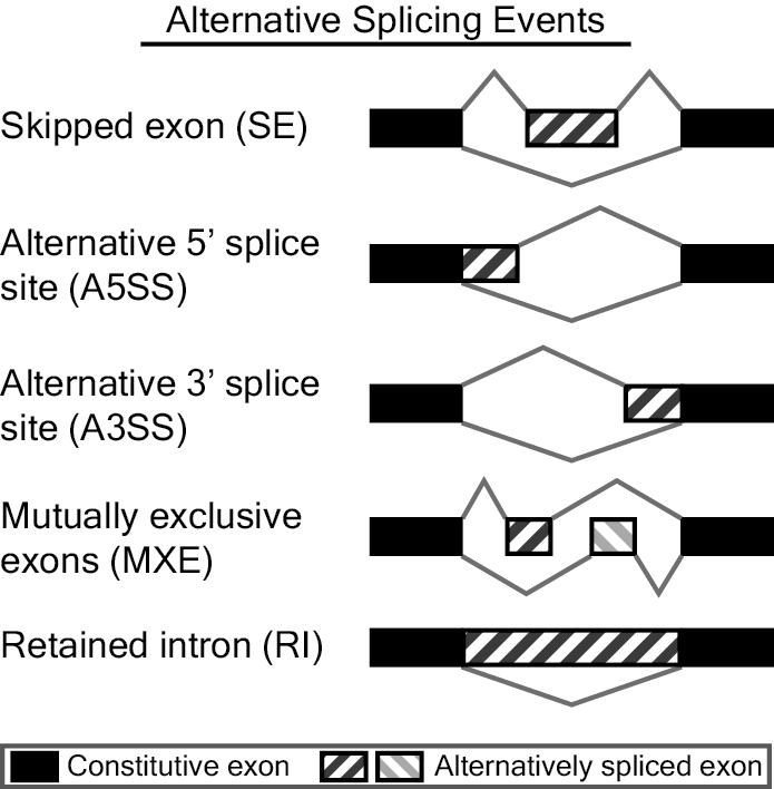
Alternative Splicing Events
MATS analyzes skipped exon (SE), alternative 5' splice site (A5SS), alternative 3' splice site (A3SS), mutually exclusive exons (MXE), and retained intron (RI) events. Possible alternative splicing
events are identified from the RNA-Seq data and annotation of transcripts in GTF format. The following is a list of provided GTF files found in the gtf directory:
Alternatively, you can download your own transcript annotation in GTF format. However, the first column (chromosome/contig name) in the GTF must match the sequence names in your bowtie index. Use bowtie-inspect (found in the bowtie directory) to display sequence names for the bowtie index.
|
|
|
|
|
Alternatively, you can download your own transcript annotation in GTF format. However, the first column (chromosome/contig name) in the GTF must match the sequence names in your bowtie index. Use bowtie-inspect (found in the bowtie directory) to display sequence names for the bowtie index.
bowtie-inspect --names your_bowtie_index
Only use a GTF in which the chromosome/contig name (first column) matches with the above command output.
Using MATS:
The following is a detailed description of the options used with MATS.
Usage:
Optional:
Examples:
Usage:
Running with fastq
Running with bam
Required Parameters:
python run_MATS.py -s1 reads1_1[,reads1_2] -s2 reads2_1[,reads2_2] -gtf gtfFile -bi bowtieIndexBase -o outDir -t readType -len readLength [options]*
Running with bam
python run_MATS.py -b1 bam_1 -b2 bam_2 -gtf gtfFile -o outDir -t readType -len readLength [options]*
| -s1 reads_1_1[,reads1_2] | FASTQ file(s) for the sample_1. For the paired-end data, two files must be in a comma separated list. (Only if using fastq) |
| -s2 reads_2_1[,reads2_2] | FASTQ file(s) for the sample_2. For the paired-end data, two files must be in a comma separated list. (Only if using fastq) |
| -b1 bam_1 | Mapping result for the sample_1 in bam format (Only if using bam) |
| -b2 bam_2 | Mapping result for the sample_2 in bam format (Only if using bam) |
| -t readType | Type of read used in the analysis. readType is either 'paired' or 'single'. 'paired' is for paired-end data and 'single' is for single-end data |
| -len <int> | The length of each read |
| -gtf gtfFile | An annotation of genes and transcripts in GTF format |
| -bi bowtieIndexBase | The basename of the bowtie indexes (ebwt files). The base name does not include the first period. For example, use hg19 for hg19.1.ebwt. (Only if using fastq) |
| -o outDir | The output directory |
| -a <int> | The "anchor length" used in TopHat. At least “anchor length” NT must be mapped to each end of a given junction. The default is 8 |
| -r1 <float> | The insert size of sample_1 data. This applies only for the paired-end data. The default is 15 |
| -r2 <float> | The insert size of sample_2 data. This applies only for the paired-end data. The default is 15 |
| -sd1 <float> | The standard deviation for the r1. The default is 70 |
| -sd2 <float> | The standard deviation for the r2. The default is 70 |
| -c <float> | The cutoff splicing difference. The cutoff used in the null hypothesis test for differential splicing. The default is 0.05 for 5% difference. Valid: 0 ≤ cutoff < 1 |
Example using fastq
python run_MATS.py -s1 testData/231ESRP.250K.r1.fastq,testData/231ESRP.250K.r2.fastq -s2 testData/231EV.250K.r1.fastq,testData/231EV.250K.r2.fastq
-gtf gtf/Homo_sapiens.Ensembl.GRCh37.65.gtf -bi ~/bowtieIndexes/hg19 -o fastqTest -t paired -len 50 -a 8 -r1 72 -sd1 40 -r2 70 -sd2 48 -c 0.05
Example using bam
python run_MATS.py -b1 testData/ESRP.bam -b2 testData/EV.bam -gtf gtf/Homo_sapiens.Ensembl.GRCh37.65.gtf -o bamTest -t paired -len 50 -c 0.05
Output:
All output files are in outputFolder
|
|
|
|
|
|
|