Install MATS:
- Add the Python 2.6 directory to the $PATH environment variable
|
- Add the NumPy and SciPy directory to the $PYTHONPATH environment variable
|
- OPTIONAL: If using the Bayesian method in MATS P value calculation, then install
JAGS (Just Another Gibbs Sampler)
|
- OPTIONAL: Add the JAGS directory to the $PATH environment variable
|
- OPTIONAL: If using createJunctionAnnotation.sh then install PYGR (Python Graph Database)
|
Run MATS:
- Run MATS in the same folder when MATS is unzipped.
|
- ./MATS.sh [-d InputDataFile] [-o OutputFolder][-c Cutoff_Splicing_Difference(default: 0.1)]
[-t Null_Hypothesis_Type(default: 1)][-p Number_of_Processors(default:1)] [-m Statistical_Method(default:B)][-s
Max_Simulation_Precision(default: 7)]
-c Cutoff_Splicing_Difference. The cutoff used in the null
hypothesis test for differential splicing or switch-like
difference.
-t Null_Hypothesis_Type. 1: null hypothesis for differential
splicing (|InclusionLevel1-InclusionLevel2|<=cutoff. 2: null
hypothesis for switch-like difference (outside of the region
(InclusionLevel1 <=cutoff and InclusionLevel2>=1-cutoff) or
(InclusionLevel1 >=1-cutoff and InclusionLevel2<=cutoff).
-p Number_of_Processors. MATS is capable of using multiple
instances. This parameter specifies the max number of
processors MATS will use.
-m Statistical_Method. B: MATS will use the Bayesian method. L: MATS will use likelihood-ratio test, which is ~100x faster than the Bayesian method.
-s Max_Simulation_Precision. This parameter is disabled for the likelihood-ratio test. It decides
the max precision MATS can reach for the P values through simulations. For example, MATS can reach the
highest precision of 10-7 for -s 7.
|
- Run the test dataset with splicing difference cutoff
10%, testing for the null hypothesis of differential
splicing |InclusionLevel1-InclusionLevel2|<=10%, using one
processor, the Bayesian method and 7 simulation rounds:
|
Input Data File Format:
Each column is TAB delimited. Input file should have the first
line as the title.
| id |
Inclusion
Junction Count Sample1 |
Skipping
Junction Count Sample1 |
Inclusion
Junction Count Sample2 |
Skipping
Junction Count Sample2 |
| 1 |
43 |
6 |
2 |
59 |
| 2 |
59 |
49 |
281 |
297 |
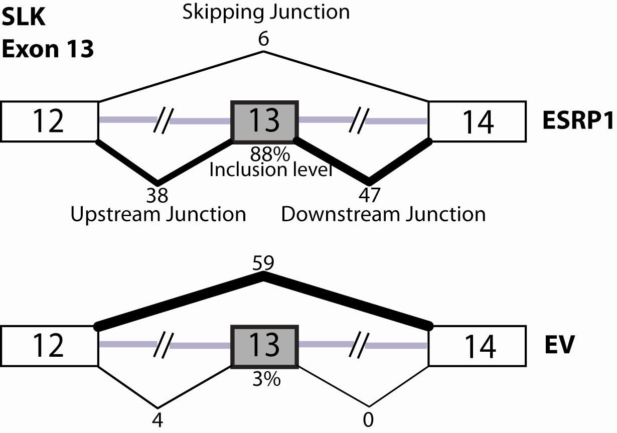
For example, when sample 1 is the ESRP1 over-expression sample
and sample 2 is the EV sample, the first line of the data file is from the figure
below. The inclusion junction count in the sample 1 is
summarized by round((38+47)/2)=43.The skipping junction count in
the sample 1 is the 6 as illustrated in the figure.
Interpret the MATS result:
The output file is a TAB delimited file named 'MATS_result.txt',
which contains the following
columns:
| id |
Inclusion
Junction Count Sample1 |
Skipping
Junction Count Sample1 |
Inclusion
Junction Count Sample2 |
Skipping
Junction Count Sample2 |
Inclusion Level Sample1 |
Inclusion Level Sample2 |
Posterior_Probability |
Posterior_P_Value |
FDR |
| 1 |
43 |
6 |
2 |
59 |
0.88 |
0.03 |
1.0 |
0.0 |
0.0 |
|
The last 3 columns of the output contain statistics for splicing difference.
- Posterior probability of splicing difference no less than a cutoff (default 10% splicing difference). High posterior probability indicates high probability of splicing difference.
|
- Posterior P value of splicing difference. Small posterior P value indicates high statistical significance of splicing difference.
|
- False discovery rate (FDR) of splicing difference. Small FDR indicates low probability of getting false discovery from the significant exons.
|
Convert SAM file to input data file:
- MATS includes a program, "convertSamToMATSInput.py", that you can use to convert SAM format output from an aligner such as Tophat to MATS input file format.
|
- Here is a detailed guide about the converting tool for SAM to MATS input. The converting tool is included in the MATS download.
|
Convert Bowtie Output to SAM file:
- We also support the Bowtie output of RNA-Seq reads mapped to annotated junctions.
|
- Here is a detailed guide about the converting tool for Bowtie output to SAM. The converting tool is included in the MATS download.
|
ESRP Dataset
The FASTQ files for the ESRP dataset
are available here: ESRP1 sample and
EV sample.
The junction annotation is available for Ensembl release 57 and UCSC Known Genes (hg19) in FASTA format. For instructions on making a bowtie index for the junction annotation, consult the bowtie manual.
The Bowtie output of the FASTQ files can be
used to generate the results of our manuscript.
Junction annotation with user defined length can also be created by following the instructions here.
Example MATS Pipeline
################################################
### Step 1. Convert bowtie output to SAM format
################################################
#
# If a user uses an aligner (other than bowtie) that creates SAM format, a user can skip this step and go to Step 2.
# Since bowtie needs to align reads to genome and junctions separately, the bowtie output must be combined before preceeding to Step 2.
#
# This example pipeline shows how to process 50bp reads with 84bp junction length.
# Since different junction lengths may be needed for different read lengths,
# a junction annotaion file (fasta) with user-defined junction length can be created using createJunctionAnnotation.sh script that comes with MATS
# For example, if a user has 32bp reads and wants to use 54bp junction length (27bp from each end of junction),
# run the following line
#
./createJunctionAnnotation.sh -d Ensembl -o Ensembl_54 -j 27 -p /Path/to/pygr/hg19/
#
# It will create junctions.Ensembl.54nt.fasta and bowtieIndex files (in *.ebwt format) in the output directory
# A user can use the resulting bowtieIndex for bowtie mapping and use fasta junction annotation file for the following process
#
# bowtie can align paired-end reads using the -1 and -2 options for pairs of fastq files
# for more information about bowtie mapping, consult bowtie manual page
# http://bowtie-bio.sourceforge.net/manual.shtm
#
### Create a sam file from genome mapping of each sample.
# bowtie output can be either single-end or paired-end
python makeSamFromBowtieOut.py ESRP.hg19.bowtie.out ESRP.hg19.sam 50 84
python makeSamFromBowtieOut.py EV.hg19.bowtie.out EV.hg19.sam 50 84
### Create a sam file from junction mapping of each sample.
# junction.Ensembl.r57.84nt.fasta is downloadable
python makeSamFromBowtieOut.py ESRP.junction.bowtie.out ESRP.junction.sam 50 84 junctions.Ensembl.r57.84nt.fasta
python makeSamFromBowtieOut.py EV.junction.bowtie.out EV.junction.sam 50 84 junctions.Ensembl.r57.84nt.fasta
#
# If a user created an annotaion file (fasta) with a user-defined junction length using createJunctionAnnotation.sh script, use the following:
#
python makeSamFromBowtieOut.py ESRP.junction.bowtie.out ESRP.junction.sam 32 54 junctions.Ensembl.54nt.fasta
python makeSamFromBowtieOut.py EV.junction.bowtie.out EV.junction.sam 32 54 junctions.Ensembl.54nt.fasta
#
### combine genome and junction sam files
cat ESRP.hg19.sam ESRP.junction.sam > ESRP_SE.sam
cat EV.hg19.sam EV.junction.sam > EV_SE.sam
#############################################################
### Step 2. make MATS input file for AS events
#############################################################
#
# make MATS input files for exon skipping events and alternative 5/3 splice site events from the sam files
# sam files are from Step 1 (using bowtie only) or an aligner that support sam format such as TopHat or SpliceMap
#
python convertSamToMATSInput.py genesAndExons.Ensembl.r57.txt ESRP_SE.sam EV_SE.sam SE ESRP EV 50 84 output
#
# It will generate following files in the output directory.
# exonSkipping.txt and MATS.input.exonSkipping.txt for exon skipping events
# altSS.txt and MATS.input.altSS.txt for alternative 5/3 splice site events
######################
### Step 3. run MATS
######################
# run MATS with MATS.input.exonSkipping.txt for exon skipping events
./MATS.sh -d MATS.input.exonSkipping.txt -o MATS_ES -c 0.1 -t 1 -p 1 -s 7
# run MATS with MATS.input.altSS.txt for alternative 5/3 splice site events
./MATS.sh -d MATS.input.altSS.txt -o MATS_ALT_SS -c 0.1 -t 1 -p 1 -s 7